General Chemistry: Lec XXVIII

Chem 1200

Angel C. de Dios

Kinetics VI

Zoom

As we near the end of the lectures on kinetics, it is important to reiterate the experimental side of kinetics. In the laboratory, the methods of initial rates require several runs for the same reaction. Each run begins with known initial concentrations of reactants. As you notice, when we do this on paper, it helps if the initial concentrations are chosen such that only one reactant is changing its concentration between runs. It is likewise helpful if this reactant is changing its concentration by an integral multiple. In the other method, where we simply monitor how a reactant is changing its concentration, it is necessary to draw test plots. We need to check which graph yields the best straight line. The test plots are [A] vs. time (zero order), square root of [A] vs. time (half order), ln[A] vs. time (first order), and 1/[A] vs. time (second order). All these plots except for the second order have a negative slope, from which we extract the rate constant. Drawing these plots is good exercise since this is how it is done in the real world. On paper, as in an exam, we will take advantage of the half-life as a clue to the order of a reaction. When we do not have time to draw all these test plots and given that the choices are limited to zero, first and second order, we can use the half-life to determine quickly the order of the reaction. In zero order, since the rate is constant, it should take shorter times to successively half the concentration of the reactant. The half-life is therefore decreasing as the reaction progresses in zero order. First order reactions are special, its half-life is constant all throughout the reaction. In second order, the rate of the reaction slows down a lot faster as the reactant is consumed thus making the successive half-lives longer. An increasing half-life as a reaction progresses therefore suggests a second order process. All of these, both test plots and using half-life as a clue, work if there is only one reactant. In the case of two reactants (like the fading of phenolphthalein), these approaches can still be applied by using one of the reactants in very large excess. This excess reactant will therefore maintain its concentration as the reaction progresses. This allows us to monitor the rate of the reaction as a function of the concentration of the limiting reactant. In this case, we will make test plots for the concentration of the limiting reactant. Whichever plot gives us a straight line provides a rate constant. But we need to keep in mind that this rate constant may still have a dependence on the concentration of the reactant in excess. That is why we call this a pseudo rate constant. We then have to repeat the experiment at different concentrations of the excess reactant to see the dependence of the pseudo rate constant on the excess reactant. The experience in the laboratory course is important since this is where you will see it first-hand, and go through the entire scheme of determining the rate law experimentally.

Now, we will look at other details of kinetics. Some of these are beyond the scope of this course (except for the temperature dependence and reaction energy diagrams). Nonetheless, these are provided to give you a fuller overview of kinetics. For example, here is a complex reaction mechanism.

Before we discuss the temperature dependence of rates of reactions, it is important to relate kinetics to what we already have learned in thermodynamics and equilibrium.

Factors that can affect rate constants

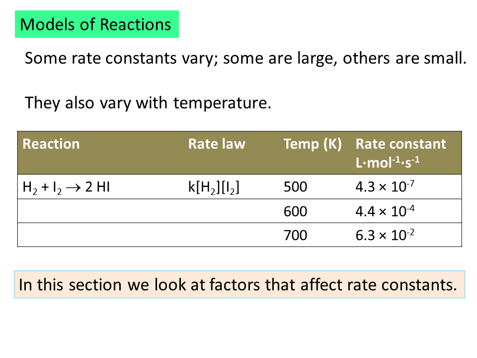
Rates of most reactions are very sensitive to temperature. Most increase rapidly with increasing temperature. A mere increase of 10 degrees, 298 K to 308 K, for example, can lead to a doubling of the reaction rate. If we recall the kinetic molecular theory (which was discussed in the previous semester of this course), one finds that the average speed of molecules increases with temperature. In fact, the average speed is related to the square root of the absolute temperature. For a reaction to occur, the participants need to collide with each other. Hence, one may suggest that as the temperature rises, the relative speeds of molecules with respect to one another increase (as the distribution of molecules among various velocities expands as the temperature is raised), leading to an increase in collision frequency. However, this is only a square root (a very mild) dependence on temperature. It does not explain why rates can double by simply raising the temperature by 10 degrees.

Here is an example:

By simply increasing the temperature by 20%, 500 K to 600 K, the rate constant increases by three orders of magnitude!

Here is another visual example:

In the above, magnesium metal is oxidized by water to form hydrogen gas, Mg²⁺ and OH^-. Phenolphthalein is added so the solution turns pink in the presence of the hydroxide ion.

Phenomenological approach

In order to understand better the temperature dependence of rates, the best way is to look closer at the observed temperature dependence. The dependence of rates on temperature manifests in the temperature dependence of the rate constant, k. By focusing on k, one has removed the concentration dependence of the rate of the reaction. In 1887, Svante Arrhenius suggested that rate constants very exponentially (This is a very strong dependence!) with the reciprocal of the absolute temperature:
The above equation is purely empirical. Our task now is to interpret what this equation means. RT is in units of energy per mole, thus, E_a is in units of energy as mole as well. A has the same units as the rate constant k. Taking the natural logarithm of both sides of the equation provides us with:
indicating that a plot of ln k versus the reciprocal of the absolute temperature, 1/T, will yield a straight line with a slope of -E_a/R and an intercept ln A.

Here is an example:

THE HYDROLYSIS OF DI-ISOPROPYL METHYLPHOSPHONATE IN GROUND WATER
Gary A. Sega¹, Bruce A. Tomkins¹, Wayne H. Griest¹, and Charles K. Bayne²
¹Chemical and Analytical Sciences Division and ²Computer Science and Mathematics Division Oak Ridge National Laboratory, Oak Ridge, TN 37831
Diisopropyl methylphosphonate is a chemical by-product resulting from the manufacture of Sarin (GB), a nerve gas that was produced by the Army in the 1950s. A chemical by-product is a chemical that is formed while making another substance. Sarin was produced and stored only in the Rocky Mountain Arsenal outside of Denver, Colorado. Production of Sarin in the United States was discontinued in 1957. Diisopropyl methylphosphonate is not known to occur naturally in the environment. It is not likely to be produced in the United States in the future because of the signing of a chemical treaty that bans the use, production, and stockpiling of poison gases. Diisopropyl methylphosphonate is a colorless liquid. Other names for it are DIMP, diisopropyl methane-phosphonate, phosphonic acid, and methyl-bis-(1-methylethyl)ester. (Agency forToxic Substances and Disease Registry - U.S. Department of Health and Human Services)

Notice that in the plot above the unit of k is per day. This is a very slow reaction and the half-life is in the order of several hundreds of years at room temperature. The slope is negative, indicating that the parameter E_a is positive, from the plot, it is found to be 109 kJ/mole. This is a huge number, an increase in temperature by 20 degrees will result in a tenfold increase in the rate. Unfortunately, the rate constants are very small to begin with, so even a tenfold increase still yields half-lives in the order of tens of years.

Let us look at one more problem that illustrates the difference between the steady-state approach and the one that assumes steps prior to the rate determining step reach equilibrium. This problem is from the homework and it examines a two step mechanism for the rearrangement of methyl isonitrile to acetonitrile.

In the "equilibrium" approach, we assume that the second step is rate-determining and that the first step simply reaches equilibrium. Thus, the overall rate is k2[A*]. Since A* is an intermediate, we need to find its expression in terms of the reactants (and products, possibly). If step 1 reaches equilibrium then k1[A][M] = k-1[A*][M], which yields [A*] = (k1/k-1)[A]. Thus, the overall rate is simply (k2)(k1/k-1)[A]. Obviously, step 1 can only reach equilibrium if there are enough A and M molecules. This assumption does not hold if the pressure (and therefore concentration) is low. For this, we need to use the more "robust" steady state approach, which assumes that [A*] reaches a steady state concentration:

rate of production of A* = rate of consumption of A*

k1[A][M] = k-1[A*][M] + k2[A*]

Therefore;

[A*] = (k1[A][M]) / (k2 + k-1[M])

The overall rate = k2[A*] = (k1k2[A][M]) / (k2 + k-1[M]).

At high pressure, k-1[M] >> k2 so the above denominator is simply k-1[M], and the overall rate simplifies to (k2)(k1/k-1)[A] (same result as the equilibrium approach). Equilibrium is possible for step1 at high pressure.

At low pressure, k2 >> k-1[M] so the denominator is now k2.

The overall rate then becomes k1[A][M]. It becomes second order. The first step essentially becomes rate determining.